Traversals

Throughout this series we've explored building various data structures such as binary search trees and graphs. Once established, these objects work like a database - managing data in a structured format. Like a database, their contents can also be explored though a process called traversal. In this essay, we'll review traversing data structures and will examine the popular techniques of Depth-First and Breadth-First Search.

Depth-First Search

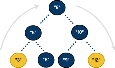
Traversals are based on "visiting" each node in a data structure. In practical terms, traversals can be seen through activities like network administration. For example, administrators will often deploy software updates to networked computers as a single task. To see how traversal works, let's introduce the process of Depth-First Search (DFS). This methodology is commonly applied to tree-shaped structures. As illustrated, our goal will be to explore the left side of the model, visit the root node, then visit the right side. Using a binary search tree, we can see the path our traversal will take:

The yellow nodes represent the first and last nodes in the traversal. The algorithm requires little code, but introduces some interesting concepts.

//depth-first in-order traversal
func processAVLDepthTraversal() {
    //check for a nil condition
    if (self.key == nil) {
        println("no key provided..")
        return
    }

    //process the left side
    if (self.left != nil) {
        left?.processAVLDepthTraversal()
    }

    println("key is \(self.key!) visited..")

    //process the right side
    if (self.right != nil) {
        right?.processAVLDepthTraversal()
    }
} //end function

At first glance, we see the algorithm makes use of recursion. With recursion, each AVLTree node (e.g. self), contains a key, as well as pointer references to its left and right nodes. For each side, (e.g., left & right) the base case consists of a straightforward check for nil. This process allows us to traverse the entire structure from the bottom-up. When applied, the algorithm traverses the structure in the following order:

3, 5, 6, 8, 9, 10, 12

Breadth-First Search

Breadth-First Search (BFS) is another technique used for traversing data structures. This algorithm is designed for open-ended data models and is typically used with graphs.

Our BFS algorithm combines techniques previously introduced including stacks and queues, generics and Dijkstra’s shortest path. With BFS, our goal is to visit all neighbors before visiting our neighbor’s, “neighbor”. Unlike Depth-First Search, the process is based on random discovery.

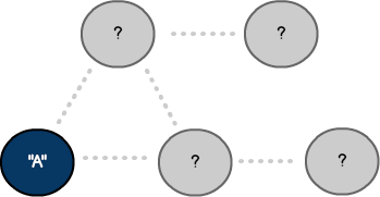
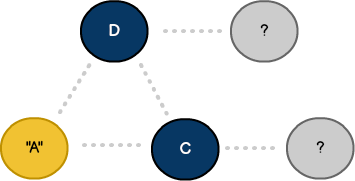
We've chosen vertex A as the starting point. Unlike Dijkstra, BFS has no concept of a destination or frontier. The algorithm is complete when all nodes have been visited. As a result, the starting point could have been any node in our graph.

Vertex A is marked as visited once its neighbors have been added to the queue.

As discussed, BFS works by exploring neighboring vertices. Since our data structure is an undirected graph, we need to ensure each node is visited only once. As a result, vertices are processed using a generic queue.

//breadth-first traversal
func traverseGraphBFS(startingv: Vertex) {
    //establish a new queue
    var graphQueue: Queue<Vertex> = Queue<Vertex>()

    //queue a starting vertex
    graphQueue.enQueue(startingv)

    while(!graphQueue.isEmpty()) {
        //traverse the next queued vertex
        var vitem = graphQueue.deQueue() as Vertex!

        //add unvisited vertices to the queue
        for e in vitem.neighbors {
            if e.neighbor.visited == false {
                println("adding vertex: \(e.neighbor.key!)")
                graphQueue.enQueue(e.neighbor)
            }
        }

        vitem.visited = true
        println("traversed vertex: \(vitem.key!)..")
    } //end while

    println("graph traversal complete..")

} //end function

The process starts by adding a single vertex to the queue. As nodes are dequeued, their neighbors are also added (to the queue). The process completes when all vertices are visited. To ensure nodes are not visited more than once, each vertex is marked with a boolean flag.