Shortest Paths

In the previous essay we saw how graphs show the relationship between two or more objects. Because of their flexibility, graphs are used in a wide range of applications including map-based services, networking and social media. Popular models may include roads, traffic, people and locations. In this essay, we'll review how to search a graph and will implement a popular algorithm called Dijkstra's shortest path.

Making Connections

The challenge with graphs is knowing how a vertex relates to other objects. Consider the social networking website, LinkedIn. With LinkedIn, each profile can be thought of as a single vertex that may be connected with other vertices.

One feature of LinkedIn is the ability to introduce yourself to new people. Under this scenario, LinkedIn will suggest routing your message through a shared connection. In graph theory, the most efficient way to deliver your message is called the shortest path.

The shortest path from vertex A to C is through vertex B.

Finding Your Way

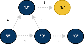
Shortest paths can also be seen with map-based services like Google Maps. Users frequently use Google Maps to ascertain driving directions between two points. As we know, there are often multiple ways to get to any destination. The shortest route will often depend on various factors such traffic, road conditions, accidents and time of day. In graph theory, these external factors represent edge weights.

The shortest path from vertex A to C is through vertex A.

This example illustrates some key points we'll see in Dijkstra's algorithm. In addition to there being multiple ways to arrive at vertex C from A, the shortest path is assumed to be through vertex B. It's only when we arrive to vertex C from B, we adjust our interpretation of the shortest path and change direction (e.g. 4 < (1 + 5)). This change in direction is known as the greedy approach and is used in similar problems like the traveling salesman.

Introducing Dijkstra

Edsger Dikjstra's algorithm was published in 1959 and is designed to find the shortest path between two vertices in a directed graph with non-negative edge weights. Let's review how to implement this in Swift.

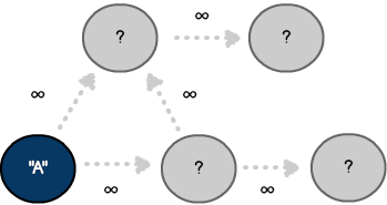
Even though our model is labeled with key values and edge weights, our algorithm can only see a subset of this information. Starting at the source vertex, our goal will be to traverse the graph.

Using Paths

Throughout our journey, we'll track each node visit in a custom data structure called Path. The total will manage the cumulative edge weight to reach a particular destination. The previous property will represent the Path taken to reach that vertex.

//maintain objects that make the "frontier"
class Path {
    var total: Int!
    var destination: Vertex
    var previous: Path!

    //object initialization
    init(){
        destination = Vertex()
    }
}

Deconstructing Dijkstra

With all the graph components in place let's see how it works. The method processDijkstra accepts the vertices source and destination as parameters. It also returns a Path. Since it may not be possible to find the destination, the return value is declared as a Swift optional.

//process Dijkstra's shortest path algorithm
func processDijkstra(source: Vertex, destination: Vertex) -> Path? {

}

Building The Frontier

As discussed, the key to understanding Dijkstra's algorthim is knowing how to traverse the graph. To help, we'll introduce a few rules and a new concept called the frontier.

var frontier: Array = Array()
var finalPaths: Array = Array()

//use source edges to create the frontier
for e in source.neighbors {
    var newPath: Path = Path()
    newPath.destination = e.neighbor
    newPath.previous = nil
    newPath.total = e.weight

    //add the new path to the frontier
    frontier.append(newPath)
}

The algorithm starts by examining the source vertex and iterating through its list of neighbors. Recall from the previous essay, each neighbor is represented as an edge. For each iteration, information about the neighboring edge is used to construct a new Path. Finally, each Path is added to the frontier.

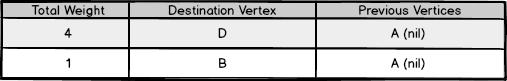
The frontier visualized as a list.

With our frontier established, the next step involves traversing the path with the smallest total weight (e.g, B). Identifying the bestPath is accomplished using this linear approach:

//obtain the best path
var bestPath: Path = Path()
while(frontier.count != 0) {
    //support path changes using the greedy approach
    bestPath = Path()

    var x: Int = 0
    var pathIndex: Int = 0

    for (x = 0; x < frontier.count; x++) {
        var itemPath: Path = frontier[x]

        if (bestPath.total == nil) || (itemPath.total < bestPath.total) {
            bestPath = itemPath
            pathIndex = x
        }
    } //end for

An important section to note is the while loop condition. As we traverse the graph, Path objects will be added and removed from the frontier. Once a Path is removed, we assume the shortest path to that destination as been found. As a result, we know we've traversed all possible paths when the frontier reaches zero.

    //enumerate the bestPath edges
    for e in bestPath.destination.neighbors {
        var newPath: Path = Path()
        newPath.destination = e.neighbor
        newPath.previous = bestPath
        newPath.total = bestPath.total + e.weight

        //add the new path to the frontier
        frontier.append(newPath)
    }

    //preserve the bestPath
    finalPaths.append(bestPath)

    //remove the bestPath from the frontier
    frontier.removeAtIndex(pathIndex)
} //end while

As shown, we've used the bestPath to build a new series of Paths. We've also preserved our visit history with each new object. With this section completed, let's review our changes to the frontier:

The frontier after visiting two additional vertices

At this point, we've learned a little more about our graph. There are now two possible paths to vertex D. The shortest path has also changed to arrive at vertex C. Finally, the Path through route A-B has been removed and has been added to a new structure named finalPaths.

A Single Source

Dijkstra's algorithm can be described as "single source" because it calculates the path to every vertex. In our example, we've preserved this information in the finalPaths array.

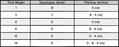
The finalPaths once the frontier reaches zero. As shown, every permutation from vertex A is calculated.

Based on this data, we can see the shortest path to vertex E from A is A-D-E. The bonus is that in addition to obtaining information for a single route, we've also calculated the shortest path to each node in the graph.

Asymptotics

Dijkstra's algorithm is an elegant solution to a complex problem. Even though we've used it effectively, we can improve its performance by making a few adjustments. We'll analyze those details in the next essay.

Want to see the entire algorithm? Here's the source.